Ray tracing: Computing ray-circle intersections

Part 1: Ray tracing: Computing ray-circle intersections
Part 2: Ray tracing: Computing ray-sphere intersections

(Code for this post is available on GitHub.)

I'm currently making my way through Ray Tracing in One Weekend, also available for free, and its 500 lines of C++ implementation. Being a bit rusty on the math side, these posts are my notes to supplement the book.

In this part and the next we focus on the most central part of a ray tracer: computing 2D line-circle and 3D line-sphere intersections. Those computations enable us to trace a ray from the eye, or camera position, through a pixel on the screen, or image plane, and into the scene. As the ray travels through the scene we want to determine if it hits, or intersects with, a scene object such as a circle or sphere, and if so at which position. If, where, and with which scene object the ray intersects determines the image plane's color at that pixel.

We start out with 2D line-circle intersection because it's simpler to visualize and because once the scalar math is worked out, it generalizes nicely to 3D line-sphere intersection and vector math. What we're working toward is illustrated in the Wikipedia article on ray tracing:

Supplementing the illustration is Disney's Practical Guide to Path Tracing, providing a humourous non-technical overview and the Painting With Light talk which adds depth and historical context.

Circle centered around origin

A circle may be defined in terms of the position of its center and its radius. To start simple, assume the circle is centered around the origin at \((0,0)\). The circle equation, or circle on standard form, then becomes $$x^2 + y^2 = r^2$$ The way to read the circle equation is that for any point \((x,y)\), if \(x^2 + y^2 = r^2\) then the point is on the circle, otherwise it's not. That follows from the Pythagorean theorem or distance formula. We can visualize the relationship between the circle equation and the Pythagorean theorem by considering a point \((x,y)\) on the circle shown below:

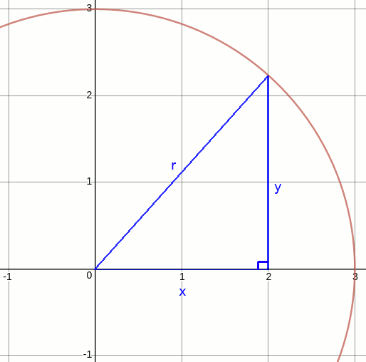
For this right-sided triangle and the point on circle, \(\sqrt{x^2 + y^2} = r\). By squaring both sides we get rid of the square root and end up with the circle equation.

Circle offset from origin

Instead of the circle centered at \((0,0)\), it may be centered at any point \((c_x, c_y)\), extending the circle equation: $$\begin{eqnarray*} (x - c_x)^2 + (y - c_y)^2 = r^2 \end{eqnarray*}$$ Say we take the circle from previously and shift its center to \((2,0)\), then points on the circle would satisfy \((2 - 2)^2 + (3 - 0)^2 = r^2\).

To keep the following examples short, we assume the circle is centered at \((0,0)\), and so \(c_x\) and \(c_y\) can be ignored.

Line and circle intersections

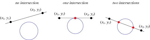
Assuming a circle \(x^2 + y^2 = r^2\) and a line \(y = ax + b\), three possible intersection scenarios exist:

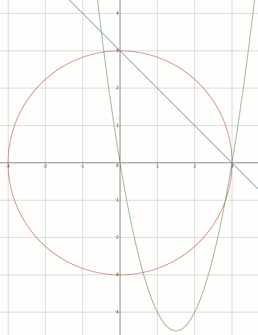
As an example, let's go with the circle \(x^2 + y^2 = 3^2\) and the line \(y = -x + 3\). If the two intersect, then for some value of \(x\) and for some value of \(y\), substituting those same values into both equations, each equation must hold. It doesn't imply that the left side of one equation equals the right side of the other, but that left and right side of each equation by itself remains equal.

Since at a point of intersection, the value of \(x\) and the value of \(y\) in the two equations must be the same, then either \(y = -x + 3\) or \(x = -y + 3\) of the line equation may be substituted into the circle equation. Substituting in \(y\) yields this new equation: $$x^2 + (-x + 3)^2 = 3^2$$ The goal of substituting one equation into the other is that instead of one circle equation with two unknowns (\(x\) and \(y\)), out comes one quadratic equation with one unknown (\(x\)): $$\begin{eqnarray*} x^2 + (-x + 3)(-x + 3) = 3^2 & & \textrm{\{expand \(y = -x + 3\)\}}\\ x^2 + x^2 - 3x - 3x + 9 = 9 & & \textrm{\{multiply out parenthesis\}}\\ x^2 + x^2 - 3x - 3x = 0 & & \textrm{\{subtract 9 from both sides\}}\\ 2x^2 - 6x = 0 & & \textrm{\{simplify\}} \end{eqnarray*}$$ Solving a quadratic equation of the standard form \(ax^2 + bx + c = 0\) for \(x\) is about determining values of \(x\) for which \(y = 0\). In other words, where the quadratic equation intersects the \(x\) axis.

The line, circle, and quadratic equations are depicted graphically below. From the graphs, it's easy to visually confirm that the solutions to the quadratic equation are \(x_1 = 0\) and \(x_2 = 3\):

The standard method for solving algebraically involves substituting the coefficients of \(ax^2 + bx + c\), that is \(a\), \(b\), and \(c\), into the equation below, with \(d\) being the discriminant: $$\begin{eqnarray*} x = \dfrac{-b \pm \sqrt{d}}{2a} \textrm{, where \(d = b^2 - 4ac\)} \end{eqnarray*}$$ The discriminant indicates which of the three intersection scenarios to expect. If \(d = 0\), then one solution, or intersection, as the square root term disappears. If \(d > 0\), then two solutions, or intersections, as the square root term must be both added and subtracted. If \(d < 0\), then no solution, or intersection, as taking the square root of a negative number is undefined:

$$d = (-6)^2 - 4(2)(0) = 36$$ Computing the discriminant only is useful only as a means to determine the number of solutions in advance. For the actual solutions, the points of intersection, the larger equation is required: $$\begin{eqnarray*} x_1 = \dfrac{-(-6) + \sqrt{36}}{2(2)} = \dfrac{6 + 6}{4} = \dfrac{12}{4} = 3\\ x_2 = \dfrac{-(-6) - \sqrt{36}}{2(2)} = \dfrac{6 - 6}{4} = \dfrac{0}{4} = 0 \end{eqnarray*}$$ Finally, inserting the values of \(x\) into either equation gets us the corresponding values of \(y\). The line equation is the simplest of the two to work with: $$\begin{eqnarray*} y_1 = -x_1 + 3 = -0 + 3 = 3\\ y_2 = -x_2 + 3 = -3 + 3 = 0 \end{eqnarray*}$$ The points of intersection of the line and the circle are at \((0,3)\) and \((3,0)\).

Summary

At first sight, the math in this post may seem like unimportant high school math. Its true power becomes evident next, when the technique is generalized from lines and circles in 2D to lines and spheres in 3D and from scalars to vectors.